

Validation of the Meteonorm algorithm chain
The validation of radiation values generated by the Meteonorm algorithm chain was carried out using quality-controlled ground measurements of radiation as a reference dataset. These measurements come from measurement networks such as BSRN and regional or national measurement networks such as SURFRAD, SOLRAD, SMHI, CIEMAT, enerMENA, or SAURAN. These measurements were quality controlled by the IEA-PVPS Task-16 Reference Solar Measurements (Forstinger, et al. 2021).
Validation of hourly GHI
The generation of hourly global horizontal radiation or GHI is tested by comparing measured hourly GHI from the reference dataset to hourly GHI values generated by Meteonorm. The hourly GHI values generated by Meteonorm are based on the measured monthly GHI values from the reference dataset. Hence, the same underlying monthly values are present in both measured and modelled GHI datasets.
The similarity of the distributions of the hourly GHI (measured vs. modelled) values was compared using the Kolmogorov-Smirnov test Integral (KSI) as described in Espinar et al. 2008. The metric KSI OVER percent (KSI %) is used as a metric of (dis)similarity.
There is excellent agreement between modelled and measured distributions at most locations. Also Meteonorm 9 shows higher agreement than the previous version Meteonorm 8.2 (see Table 1 and Figures 1 and 2).
Table 1: Comparison of the evaluation of the distribution of generated hourly GHI compared to observed distributions using the KSI Over % score. The comparison is shown for Meteonorm 9 (MN9) and Meteonorm 8.2 (MN8.2). Lower values signify better agreement.
| Site | Year | KSI Over % Meteonorm 9 | KSI Over % Meteonorm 8.2 |
|---|---|---|---|
| Bondville, BON (US) | 2015 | 12.7 | 33.2 |
| Cabauw, CAB (NL) | 2017 | 9.2 | 26.8 |
| Gobabeb, GOB (NA) | 2015 | 3.0 | 26.0 |
| Lauder, LAU (NZ) | 2016 | 13.7 | 46.7 |
| Payerne, PAY (CH) | 2018 | 18.2 | 53.0 |
| Rock Springs, ROS (US) | 2016 | 11.7 | 22.8 |
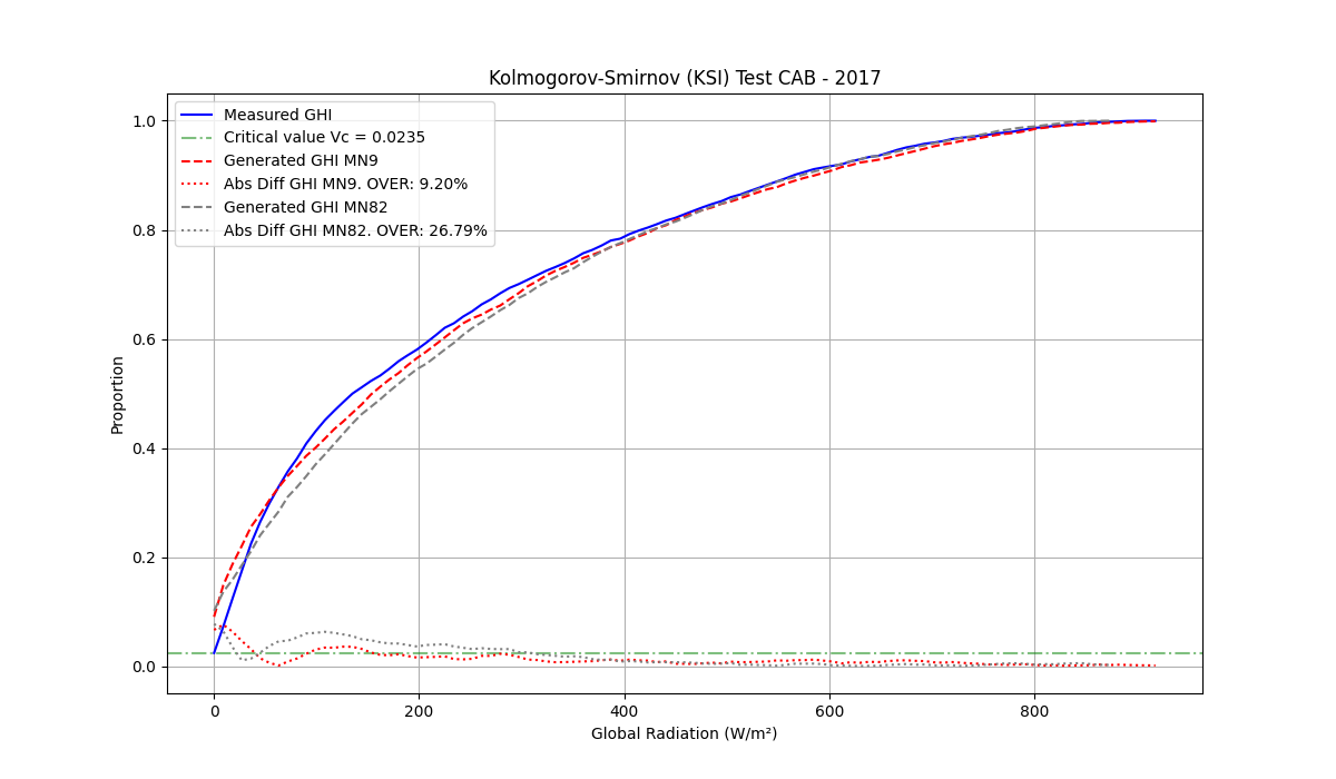
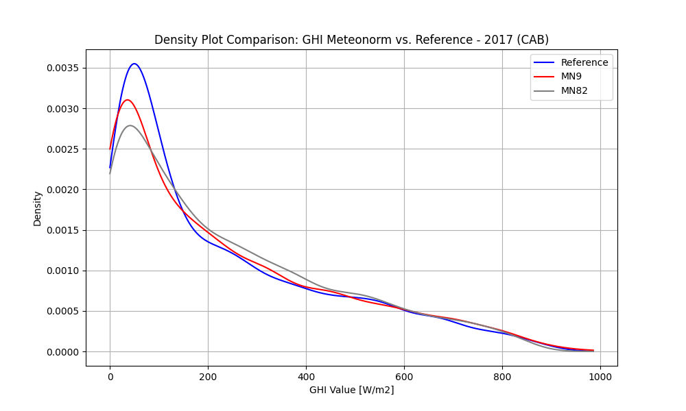
Figure 1: Examples of the cumulative distribution function and KSI % results (top) as well as distribution function (bottom) at reference location Cabauw/CAB (NL) of hourly GHI values (generated from monthly GHI). The figure shows the measured reference distributions (blue) as well as modelled distributions from Meteonorm 9 (red) and Meteonorm 8.2 (grey).
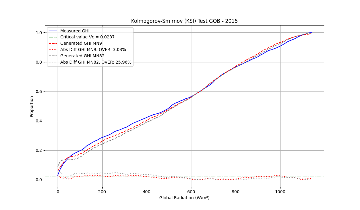
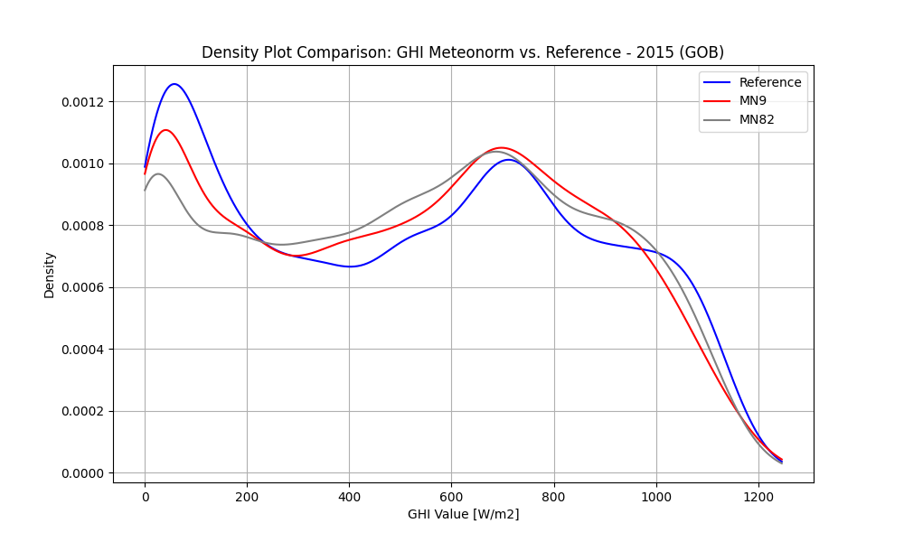
Figure 2: Examples of the cumulative distribution function and KSI % results (top) as well as distribution function (bottom) at reference location Gobabeb/GOB (NA) of hourly GHI values (generated from monthly GHI). The figure shows the measured reference distributions (blue) as well as modelled distributions from Meteonorm 9 (red) and Meteonorm 8.2 (grey).
Validation of hourly DNI
Direct normal irradiance (DNI) is tested in two approaches. Measured monthly and hourly GHI values from the reference dataset are used as inputs for the generation of hourly DNI values. Then the modelled DNI values are compared to the measured values.
MBE and RMSE for hourly DNI generated from hourly GHI
From hourly measured GHI, the generation of hourly DNI is examined, by comparing hourly measured DNI against this modelled hourly DNI. The average mean bias error (MBE), the root mean square error (RMSE), and the distribution of DNI values are examined.
The MBE is generally low and shows a slight positive bias of the Meteonorm DNI data. The RMSE is in the order of 75 to 105 W/m2 depending on the location.
Table 2: Mean bias error (MBE) and root mean square error (RMSE) between generated hourly DNI compared to observed values.
| Site | Year | MBE [W/m2] | relative RMSE [%] |
|---|---|---|---|
| Bondville, BON (US) | 2015 | 31.7 | 28.2 |
| Cabauw, CAB (NL) | 2017 | 25.5 | 41.4 |
| Gobabeb, GOB (NA) | 2015 | 16.2 | 12.6 |
| Lauder, LAU (NZ) | 2016 | 3.9 | 24.3 |
| Payerne, PAY (CH) | 2018 | 28.8 | 24.0 |
| Rock Springs, ROS (US) | 2016 | 2.3 | 26.2 |
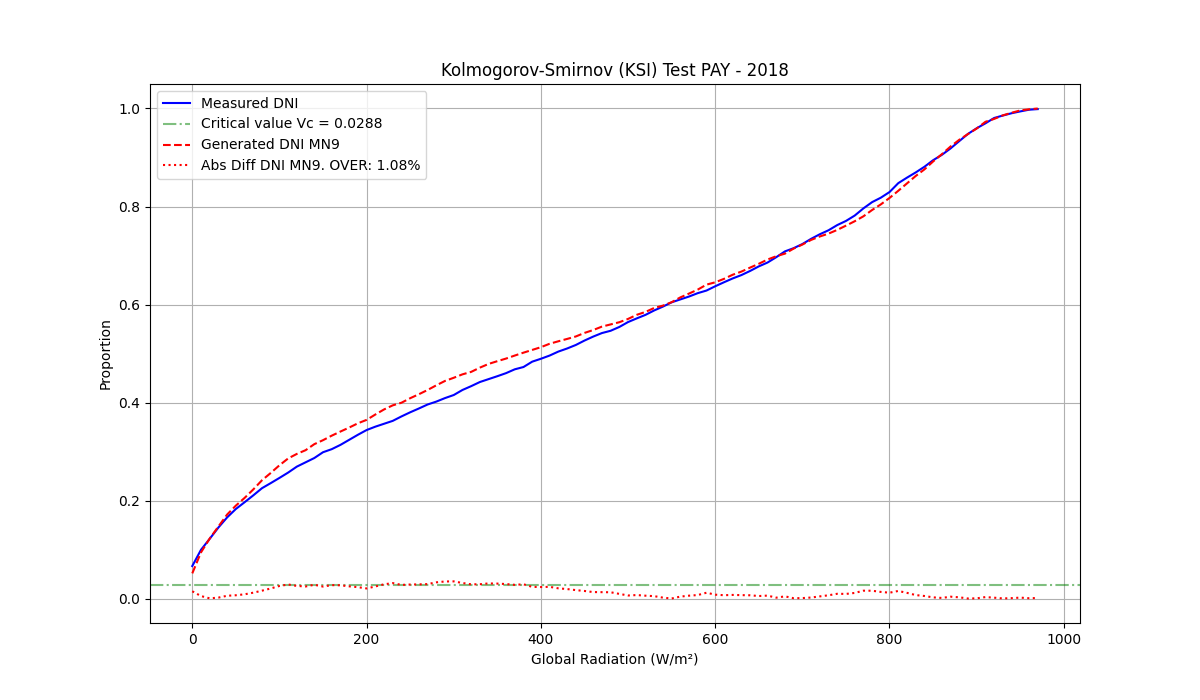
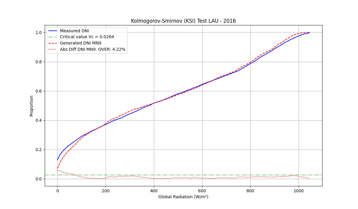
Figure 3: Examples of the cumulative distribution function and KSI % results at reference locations Payerne/PAY (CH) (top) and Lauder/LAU (NZ) (bottom). The figure shows the measured reference distributions (blue) as well as modelled distributions from Metenorm 9 (red).
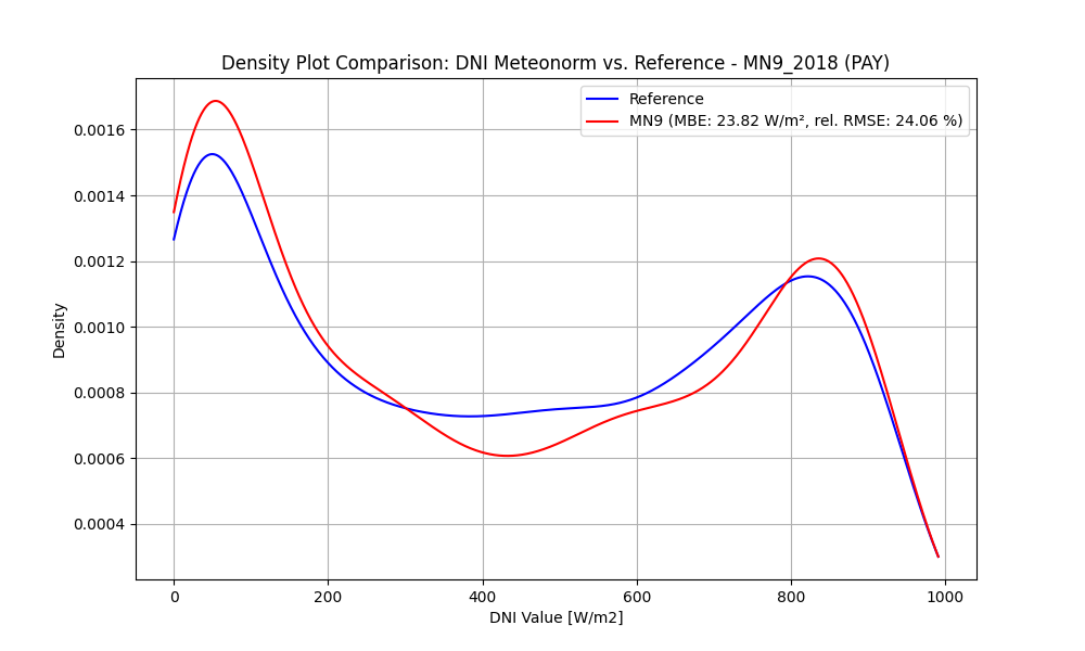
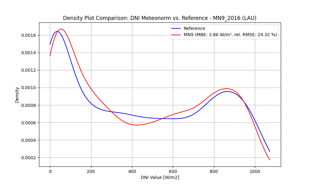
Figure 4: Examples of the distributions of hourly DNI values (generated from hourly GHI) at reference locations Payerne/PAY (CH) (top) and Lauder/LAU (NZ) (bottom). The figure shows the measured reference distributions (blue) as well as modelled distributions from Meteonorm 9 (red).
Comparing yearly DNI averages from hourly DNI generated from monthly GHI
This comparison is carried out over many stations and multiple years. The modelled hourly DNI time series are averaged to yearly values and compared to measured yearly averages.
The model performance has been tested at 41 high quality sites with one to multi year measurements by investigating the yearly means of generated beam irradiances (Table 3). The results show good agreement between the yearly averages. There is a slight positive bias in the DNI modelled by Meteonorm 9 compared to the measured values with an average relative difference of 3.32% (RMSE of 6.57%).
Table 3: Table showing the comparison of multi-year means of modelled and measured DNI values.
| Reference-Site | Years | MN9 - Modelled DNI [kWh/m2] | Reference - Measured DNI [kWh/m2] | Difference [kWh/m2] | Difference [%] |
|---|---|---|---|---|---|
| Alexander Bay (ALE) | 2016, 2017 | 3004 | 2954 | 50 | 1.69 |
| Tucson (ARI) | 2015, 2017 | 2753 | 2651 | 102 | 3.85 |
| Bahawalpur (BAH) | 2015 | 1313 | 1273 | 40 | 3.14 |
| Bondville (BON) | 2015, 2016, 2017, 2018 | 1570 | 1546 | 24 | 1.55 |
| Boulder (BOU) | 2015, 2016, 2017, 2018 | 2100 | 2021 | 79 | 3.91 |
| Cabauw (CAB) | 2015, 2016, 2017 | 1156 | 987 | 169 | 17.12 |
| Cairo (CAI) | 2015 | 2149 | 1934 | 215 | 11.12 |
| Carpentras (CAR) | 2015, 2016, 2017 | 1985 | 2055 | -70 | -3.41 |
| Cener (CEN) | 2015, 2016, 2017 | 1720 | 1637 | 83 | 5.07 |
| Chileka Airport (CHI) | 2017 | 1594 | 1558 | 36 | 2.31 |
| De Aar (DEA) | 2016, 2017, 2018 | 2800 | 2961 | -161 | -5.44 |
| Desert Rock (DES) | 2015, 2016, 2017, 2018 | 2908 | 2822 | 86 | 3.05 |
| Dar es Salaam (DAR) | 2016 | 1590 | 1470 | 120 | 8.16 |
| Fort Peck (FOP) | 2016, 2018 | 1850 | 1653 | 197 | 11.92 |
| Alice, University of Fort Hare (FOR) | 2018 | 2058 | 2126 | -68 | -3.2 |
| Fukuoka (FUK) | 2015, 2016, 2017, 2018, 2019 | 1038 | 1129 | -91 | -8.06 |
| Gaborone (GAB) | 2015, 2016 | 2513 | 2458 | 55 | 2.24 |
| Gobabeb (GOB) | 2015 | 2964 | 2902 | 62 | 2.14 |
| Ishigakijima (ISH) | 2015, 2016, 2017, 2018, 2019 | 1095 | 1082 | 13 | 1.2 |
| Langley Research Center (LAN) | 2017, 2018 | 1555 | 1602 | -47 | -2.93 |
| Las Vegas (LAS) | 2016, 2017, 2018 | 2803 | 2669 | 134 | 5.02 |
| Lauder (LAU) | 2016, 2017 | 1784 | 1690 | 94 | 5.56 |
| Milan (MIL) | 2016 | 1386 | 1375 | 11 | 0.8 |
| Minamitorishima (MIN) | 2015, 2016, 2017, 2018, 2019 | 1937 | 1930 | 7 | 0.36 |
| Norrköping (NOR) | 2015, 2016, 2017, 2018 | 1291 | 1198 | 93 | 7.76 |
| Oak Ridge (OAK) | 2015, 2016, 2017, 2018 | 1184 | 1346 | -162 | -12.04 |
| Eugene (ORE) | 2017, 2018 | 1549 | 1466 | 83 | 5.66 |
| Palaiseau (PAL) | 2017, 2018 | 1317 | 1163 | 154 | 13.24 |
| Edinburg UTRGV SRL (PAN) | 2016, 2017, 2018 | 1630 | 1587 | 43 | 2.71 |
| Payerne (PAY) | 2015, 2016, 2017, 2018 | 1523 | 1359 | 164 | 12.07 |
| Pretoria (PRE) | 2015, 2016, 2017, 2018 | 2366 | 2295 | 71 | 3.09 |
| Rock Springs (ROS) | 2015, 2016, 2017, 2018 | 1306 | 1243 | 63 | 5.07 |
| Sapporo (SAP) | 2015, 2016, 2017, 2018, 2019 | 1141 | 1054 | 87 | 8.25 |
| Sioux Falls (SIO) | 2015, 2016, 2017 | 1768 | 1653 | 115 | 6.96 |
| SRRL BMS (Colorado) (SRR) | 2015, 2016, 2017, 2018 | 2082 | 2031 | 51 | 2.51 |
| Stellenbosch (STE) | 2015, 2016 | 2284 | 2345 | -61 | -2.6 |
| Tabernas (TAB) | 2016, 2017, 2018, 2019 | 2417 | 2350 | 67 | 2.85 |
| Tataouine (TAT) | 2015 | 2309 | 2228 | 81 | 3.64 |
| Toravere (TOR) | 2015, 2016, 2017, 2018 | 1171 | 1061 | 110 | 10.37 |
| Vuwani (VUW) | 2016, 2017, 2018 | 1769 | 1746 | 23 | 1.32 |
| Windhoek (WIN) | 2017, 2018 | 2698 | 2747 | -49 | -1.78 |
| Bias (%) | 3.32 | ||||
| RMSE (%) | 6.57 |
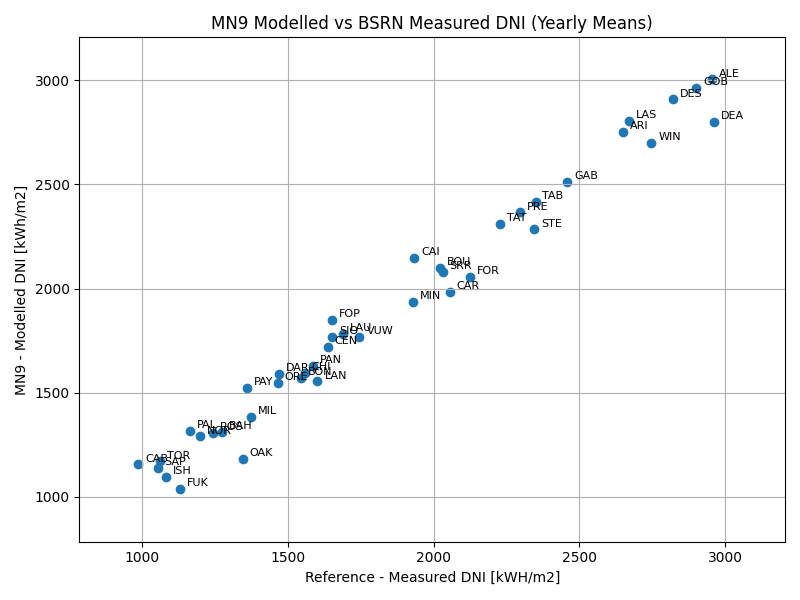
Figure 5: Scatter plot showing the comparison of multi-year means of modelled and measured DNI values. Short names correspond to the station names in the Table 3 above.